Designing neural networks: zero to micrograd

🌱 Writing a minimalist neural network from scratch is a perfect way to get to know your way around the essential components. 🌱

A while ago, I discovered Andrej Karpathy’s tiny neural net - micrograd - and, as a prelude to implementing it in Rust, I drafted my own Python version. With micrograd being intentionally minimalist, my naive neural net omits anything not absolutely required. (For example, no matrices¹ or attention layers².)

micrograd’s minimalism belies the depth of the representations it contains. We can learn more about those by exploring key design decisions baked into micrograd: What’s the rationale behind micrograd’s specific network topology? What constraints motivate its learning algorithm? And which of those are pragmatic vs essential for theoretical foundations to hold?

This summary signposts the path from early network models of the brain through to micrograd’s core design choices, some of which apply to artificial neural networks more broadly. I’ve tried to make it accessible to non-experts.

TL;DR

Our goals here are to establish:

• why micrograd implements a multilayer perceptron model
• how efficiency considerations influence the learning feedback loop
• why backpropagation and gradient descent are pragmatic design choices

In the spirit of micrograd, this write up is nominally minimalist and leaves a lot out³.

Onward. Let’s start by establishing a foundation for using physiological neural nets as a basis for designing artificial neural networks.

Why neural nets?

Humans naturally accumulate a wide variety of knowledge and develop a plethora of skills. In contrast, traditional computing requires explicit instructions to perform pre-designated tasks. It can’t self-improve or develop general abilities. There’s a chasm between traditional computing and human learning, and we’d like to make some headway toward crossing it.

A machine that has the ability to even contemplate answering a random question or performing a random task might seem like it’s thinking. This probably rings especially true when the path from input to the expected response doesn’t have an algorithmic solution. Where does one begin, though, on the design of a machine intended to execute general tasks?

The machinery for human thought is concentrated in the brain, making it natural to at least consider exploring designs based on the brain. So, let’s begin with simplified models of neuronal networks.

Cognition / connection

In the early 1940s, researchers working on mathematical models of cognition developed connectionist networks, an early form of artificial neural network that merged statistical methods with physiologically-inspired structure and function. Eventually, feedback was added to iteratively improve performance, emulating learning: the machine’s abilities improved without human intervention.

A machine with the capacity to self-improve was a huge step forward. A significant break from traditional computing was the key innovation: the code didn’t include explicit instructions for how to process inputs (i.e., how to perform any particular task). Instead, the artificial neural network’s code nudged it to develop skills.

Indeed, in its initial state, an artificial neural network (ANN) is not very capable. To develop skills, it responds to feedback about its performance. For each training epoch, the ANN accepts a challenge, produces an output, listens for feedback on the results, then updates itself to try to do better. Each of the challenges comes from training data, and the quality of that dataset is as essential as you’d expect it to be. We’re going to set that aside as an externality, though, so we can focus exclusively on model design.

Let’s take a closer look at how this fundamentally different approach to computation might be implemented, starting with cues taken from network models of the brain.

IRL neurons

The thinking machinery of the brain is impossibly complicated, but we’re going to focus exclusively on the networks formed by neurons. What can we take from those to build our own, in silico?

To oversimplify drastically: Neurons in the brain receive and modulate an input signal, then decide whether to propagate a modulated response. A neuron’s axons and synapses deliver outgoing signal to one or more downstream neurons. Generally, the idea is that each neuronal network includes a feedback circuit that influences collective network behavior. That network-level adaptive behavior is key to thinking and learning.

Figure 1.

Modeling a neural network

Based on a simplified model of the brain, an ANN is represented as a network. A network has individual entities (nodes) connected by channels (vertices, or edges); in a network model of the brain, the individual entities are neurons and the connection channels are synapses.

The perceptron model paved the way for implementing neuron behaviors, and the development of multilayer perceptron (MLP) networks built on that to add networking capabilities.

Figure 2.

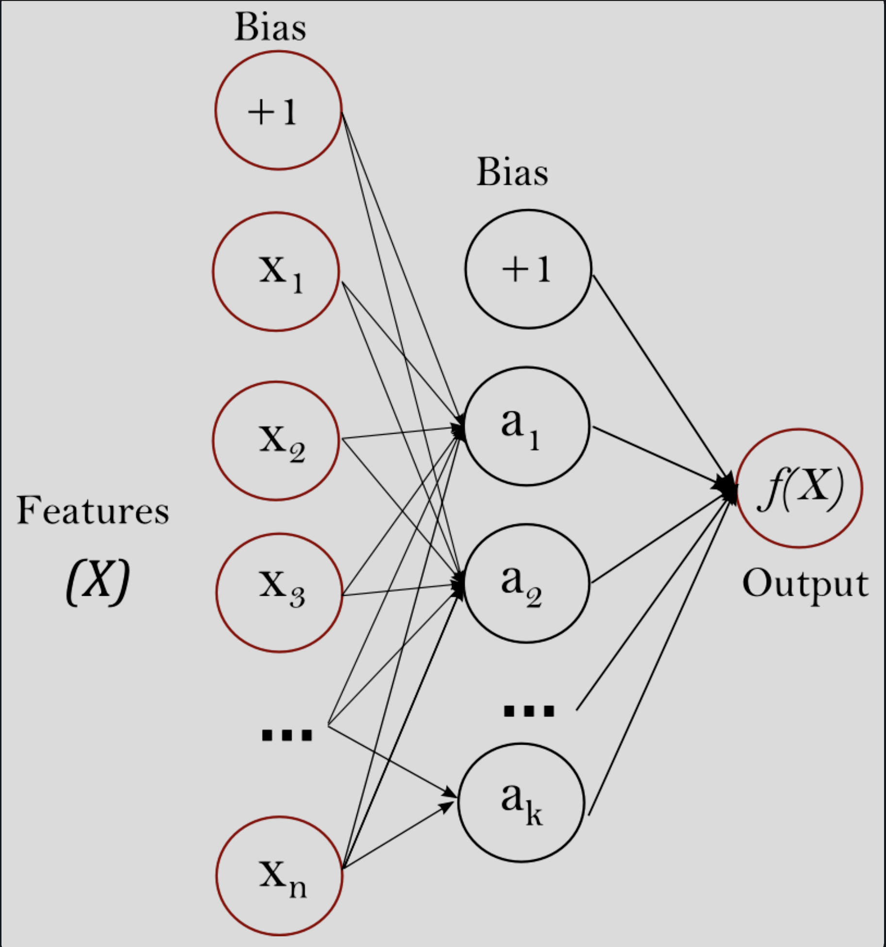
The multilayer perceptron network mimics:

1. neurons’ ability to perceive a stimulus and respond
2. neuron activation to transmit an outgoing signal
3. multiplexing neuronal activity across neuron layers

MLP topology is quite specific: nodes in a layer are not connected, and all nodes in a layer connect to each node in the next layer. Functionally, each neuron in an MLP independently perceives an input and decides whether to propagate a corresponding output to the subsequent layer in the network.

Design choice 1: Use multilayer perceptron networks.

Modeling learning

To facilitate learning, the MLP model gets a feedback loop so neurons can update. The individual neurons thus participate in coordinated collective behavior to improve network performance.

That coordinated network behavior involves an iterative process: measure forward-pass network performance, deliver feedback to neurons, update individual neurons, repeat. That’s the 10,000-foot view, at least. We’ll look into the specifics next, keeping in mind that neurons manage two signal streams:

1. information originating from the initial input to the network, received via prior-layer neurons: this is the forward pass signal
2. network performance information, received from the network output: this is the feedback signal

The learning algorithm

We can roughly model the ANN learning process as a feedback circuit.

Figure 3.

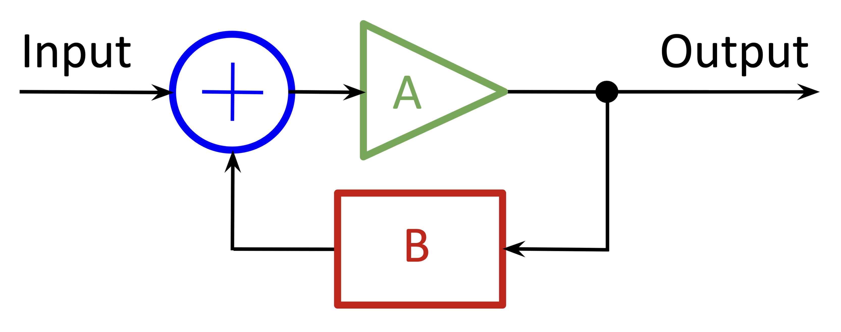
In the schematic, $A$ represents the transfer function of the forward pass through the ANN, and $B$ represents the feedback that facilitates skill development, or learning.

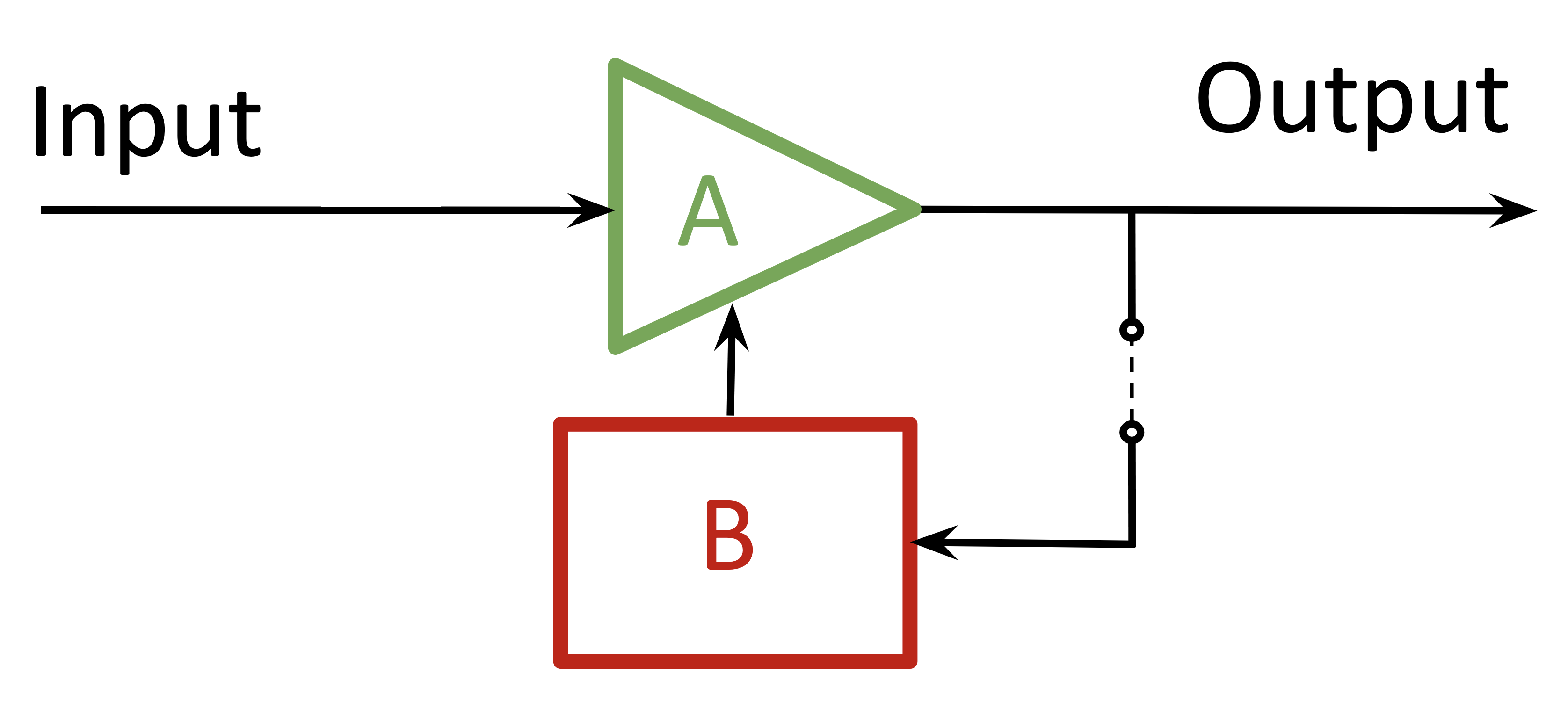
Unlike a continuous-signal circuit, the ANN processes an input separately from responding to feedback; there’s no mixing. The ⊕ represents model parameter updates between training inputs.

Better learning through efficiency

We might expect the network transfer function to be pretty complicated - the MLP structure makes that hard to avoid. On the other hand, neuron transfer functions are relatively simple. That simplicity translates to faster processing, which is consequential: a model that takes excessively long to run won’t be useful, and a model that trains slowly will receive less training and take a performance hit.

According to our MLP network model, neurons’ overall transfer functions represent two distinct stages of processing. The first stage, we’ll refer to as multiplexing - that’s where the prior layer’s outputs are combined. The second, we’ll refer to as activation.

Multiplexing in MLPs is a purely linear transformation. That linearity means the transformation is fully characterized by its scalar coefficients. We’ll call those the neuron parameters: $w$ for weights and $b$ for biases. The multiplexed output is:

$\boxed{multiplexed = ( w * neuron\_input ) + b}$

To have generalized capabilities, our network needs to include nonlinear processing on the forward pass (see the universal approximation theorem⁴ for neural networks⁵).

Corollary (requirement) to DC1: Include nonlinear component(s) in the forward pass.

After multiplexing, then, we’ll apply a nonlinear activation function before broadcasting the neuron’s output to the next layer. Leaning into how signals are propagated by brain neurons via activation thresholds and action potentials, we’ll select activation functions that mimic this behavior⁶.

Design choice 2: Use nonlinear activation functions that mimic neuronal signal propagation.

The nonlinear activation function is applied to the multiplexed signal, generating the post-activation neuron output:

$\boxed{neuron\_out = activation ( multiplexed )}$

A note about matrices, since they figure so prominently in machine learning and we’re not including them in micrograd. Same-layer neurons in MLP networks aren’t connected: they act independently. Combining this independence with linear multiplexing means we can use matrices to efficiently parallelize those computations. Also, network inputs are processed independently so they can be run through the network in parallel, too. Together with innovations in GPUs and TPUs, this makes it possible to scale models to very large numbers of parameters (currently, hundreds of billions) while training on many inputs simultaneously.

For micrograd, we won’t be parallelizing anything, but we’ll still be able to take advantage of the linearity condition. (Remember - the goal with micrograd is to build from scratch. The fewer arithmetic operations we need to implement, the better.)

Backpropagation & gradient descent

We’ve yet to define exactly how to compute neuron updates. Let’s start by clarifying what, exactly, will be updated.

Recall that neurons process inputs in two stages: multiplexing and activation. Multiplexing is linear, activation is nonlinear. It’s somewhat circular but - once we identify it - our learning algorithm will be easier to tune if the updates act on linear functions. So, we’ll restrict those to neuron parameters - i.e., the weights and biases.

Design choice 3: Use feedback to update weights and biases between training passes.

Let’s itemize structural components needed to support the learning process; this will give us a sense of implementation options. Generally, we’ll need:

1. a feedback path that connects network output to individual neurons
2. a function to evaluate network performance
3. a function to update neuron parameters

A hidden layer neuron will have multiple input-to-output paths passing through it. We’ll create a topological map of the neurons traversed on each forward path to set up the feedback paths.

Next, the loss function. Its purpose is to quantify the difference between actual and ideal outcomes during training, so the choice of metric depends on the model objectives. In alignment with micrograd’s minimalist ethos, we’ll use the basic mean square error (aka Euclidean distance, or L2 norm)⁷:

$\boxed{error = \sqrt{(actual - expected)^2}}$

Design choice 4: Use mean square error as the loss metric for micrograd.

Finally, the update function needs to tie that metric to individual neurons. This is the exciting part because we’re going to establish how our network learns.

It’s not actually obvious a priori that there’s a single update function that, when applied to all neurons, will improve network performance. Having a single function is important for streamlining model scaling and for computational efficiency, so let’s see what we can come up with.

Ideally, we’d identify a functional relationship between changes to individual neurons and network output. Given that we have a topological map, evaluating (partial) derivatives of the loss with respect to each path-neuron should give us what we need: each local gradient would represent a neuron’s influence on the loss.

The loss surface’s minimum would be located at the lowest point of a valley. To minimize the loss, individual neurons could be nudged down their respective gradients, with neurons on steeper slopes effectively being nudged further that those on shallower slopes.

Figure 4.

Let’s implement that. To get the partial derivatives, we’ll apply the chain rule backward through each path in the topological map. First, though, we need to make sure the paths are differentiable.

Expanding the neuron transfer function, we get:

$\boxed{neuron\_out = activation ( ( w * neuron\_input ) + b )}$

That’s one neuron. Same-layer neurons act independently; they’re never in the same feedback path. According to the MLP model, a neuron’s output then either becomes a next-layer neuron input or it contributes to network output. Either way, aside from activation functions⁸, forward pass processing is linear.

This is really promising. Since linear functions are always differentiable, what remains is to make sure our activation functions are differentiable, too. Potential candidates like sigmoids are both differentiable and compress inputs to mimic the effects of activation thresholds and action potentials. Let’s stick with differentiable activations⁹.

Design choice 5: Use backpropagation and gradient descent as the learning function.

Corollary to DC5: Use differentiable activation functions.

We now have a learning process for our network. We’ll iterate over our topological map, computing path-wise partial derivatives to get local gradients. For each neuron, we’ll update its parameters in proportion to the sum¹⁰ of its path-specific local gradients.

This specific method of computing local gradients and using those to determine network parameter updates is called stochastic gradient descent¹¹. It’s an intuitive approach to propagating loss feedback so that neurons are updated proportionally to their influence.

Let’s make gradient descent a little more concrete by computing an example update for a neuron, $u$, that contributes to two paths in the network.

Figure 5.

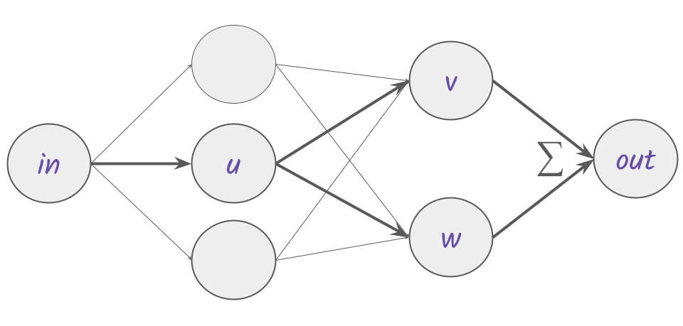
Apply the chain rule to get partial derivatives for each path:

u-v path partials: $\boxed{\partial out_{uv} / \partial in = \partial out / \partial v * \partial v / \partial u * \partial u / \partial in}$

u-w path partials: $\boxed{\partial out_{uw} / \partial in = \partial out / \partial w * \partial w / \partial u * \partial u / \partial in}$

To compute the update for $u$, we’ll only need the gradients between $out$ and $u$. The partials represent local steepness so are scaled by a global step size¹², $step$. Finally, summing over all paths that include $u$, we evaluate the total update for $u$:

$\boxed{\varDelta u = step * ((\partial out / \partial v * \partial v / \partial u) + (\partial out / \partial w * \partial w / \partial u))}$

These values are computed for each neuron, and for each path to which the neuron contributes. The process is repeated for the number of training iterations we set (or until a performance target is reached). For billions of parameters, the computational lift is significant and we can begin to see why efficiency optimizations are important.

Backpropagation using gradient descent has been remarkably successful. So successful that, despite its inherent simplicity and potential pitfalls¹³, learning facilitated by this method plus the basic MLP structure of micrograd are retained in (far more complex) state of the art models.

Aside: Model interpretability

For mere mortals, the concept of learning generally involves reasoning. Throughout, we’ve been using the term learning to represent the ANN’s performance improvements. Has the network been reasoning, in any sense that we could appreciate? Is it capable of reasoning independently once trained? The network’s transfer function post-training may not have any clear interpretation in the sense of reflecting a logical ’thought’ process. Could we figure out how the model thinks? Research on model interpretability aims to reveal the meaning in models’ (hidden-layer) tactics.

State of the art ANNs

Researchers working on machine learning didn’t land on MLPs with gradient descent as the secret sauce right off the bat. Here’s a detailed timeline of machine learning according to Wikipedia, but we’ll skip straight to the present.

The announcement for the 2024 Nobel Prize in Physics includes a very readable overview of the development of ANNs, with a focus on the progression from Hopfield networks to restricted Boltzmann machines, an important precursor to today’s mainstream machine learning models.

Many varieties of ANNs can perform high quality general purpose computation. From a theoretical perspective, the fundamental requirement for such broad capabilities is having at least one hidden layer: the network must be deep (see the universal approximation theorem⁴ for neural networks⁵).

Corollary (requirement) to DC1: At least one hidden layer.

In practice, a very large number of nodes and many training iterations on large and varied datasets are required. For decades, the scale of available training data and compute power limited both research and adoption of ANNs. Eventually, massive datasets became available for training, and realistic training times for models of sufficient size and complexity were made possible by advances in GPUs.

This unblocked progress, and rapid development ensued. Today, ANNs power large language models (LLMs) such as Anthropic’s Claude, Meta’s Llama, Google’s Gemini, OpenAI’s GPT-x series and o1. An example mainstream application that uses such a model is Google’s NotebookLM. It fine tunes its base model on data you share with it - maybe a research paper or a thesis, though needn’t be research-y at all. The end result is a podcast with two ‘people’ discussing your input data - occasionally with decent results, though not always. Case in point, a podcast that was fine tuned on this post. The discussion strays from developing the rationale behind micrograd design, ultimately covering a range of AI topics of varying degrees of relevance.

Believe it or not, the fundamental elements of the ANNs driving these advanced models build on analogous components present in our super-simple micrograd ANN. For a peek at implementing micrograd’s components in code and seeing them in action - model training and eval - here’s a write up of my version.

Design choices - list summary

Extracting the specific choices that’ll set the stage for implementing micrograd:

• Use multilayer perceptron networks.

  • Corollary requirement: At least one hidden layer.
  • Corollary requirement: Include nonlinear component(s) in the forward pass.

• Use nonlinear activation functions that mimic neuronal signal propagation.

• Use feedback to update weights and biases between training passes.

• Use backpropagation and gradient descent as the learning algorithm.

  • Corollary: Use differentiable activation functions.

• Use mean squared error as the loss metric.

What’s missing from micrograd?

A minimalist implementation of an ANN works surprisingly well. It’s also missing some elements that really should be included in any non-trivial model.

Efficient processing

In reality, the sort of training that LLMs require isn’t even possible without pulling out every stop on efficiency. At the very least, we need to use matrices to leverage linearity and independence. Incorporating PyTorch or Keras, and supporting libraries such as Einsum and Jax, is essentially necessary to train a non-miniature ANN. Taking it a step further - for production-grade models, GPU optimization is critical.

Tokenization

Tokenization involves tactical groupings of fractional components of inputs. This is applied as preprocessing of the input data, and can boost performance by starting from a more semantically robust kernel.

Model evaluation

A trained model might have satisfied the loss function tolerance, but will it perform well on data not in the training dataset? Post-training performance testing is important for assessing accuracy/correctness and also alignment. Many swear by their own custom eval processes, but you might want to start with Hugging Face’s guide, or with the cute and approachable Forest Friends eval guide.

Beyond micrograd

State of the art ANNs are significantly more complex than micrograd, and include innovative elements which improve performance and/or efficiency.

Notably, the transformer architecture is one of the great successes in the past decade of advances in machine learning. The original paper, Attention is all you need, is well worth reading.

A few other starting points for further investigation - definitely not comprehensive.

• More . transformer . resources
• Transformer cicuits
• Reinforcement learning
• Retrieval augmented generation
• Long term short memory
• Convolutional neural networks
• Recurrent neural networks
• Generative adversarial networks
• Decision transformers